Discrete stochastic Erlang epidemic model
Author: Lam Ha @lamhm
Date: 2018-10-03
Load Packages for Julia
using DataFrames
using Distributions
using Plots
Calculate Discrete Erlang Probabilities
The following function is to calculate the discrete truncated Erlang probability, given $k$ and $\gamma$:
\begin{equation} p_i = \frac{1}{C(n^{E})} \Bigl(\sum_{j=0}^{k-1} \frac{e^{-(i-1)\gamma} \times ((i-1)\gamma)^{j}} {j!} -\sum_{j=0}^{k-1} \frac{e^{-i\gamma} \times (i\gamma)^{j}} {j!}\Bigr),\quad\text{for $i=1,…,n^{E}$}. \end{equation}
where
\begin{equation} n^{E} = argmin_n\Bigl(C(n) = 1 - \sum_{j=0}^{k-1} \frac{e^{-n\gamma} \times (n\gamma)^{j}} {j!} > 0.99 \Bigr) \end{equation}
N.B. The formula of $p_i$ here is slightly different from what is shown in the original paper because the latter (which is likely to be wrong) would lead to negative probabilities.
#' @param k     The shape parameter of the Erlang distribution.
#' @param gamma The rate parameter of the Erlang distribution.
#' @return      A vector containing all p_i values, for i = 1 : n.
function compute_erlang_discrete_prob(k::Int64, gamma::Float64)
    n_bin = 0
    factorials = zeros(Int64, k + 1)
    factorials[1] = 1  ## factorials[1] = 0!
    for i = 1 : k
        factorials[i + 1] = factorials[i] * i  ## factorial[i + 1] = i!
    end

    one_sub_cummulative_probs = Float64[]
    cummulative_prob = 0
    while cummulative_prob <= 0.99
        n_bin = n_bin + 1
        push!(one_sub_cummulative_probs, 0)

        for j = 0 : (k - 1)
            one_sub_cummulative_probs[end] =
                one_sub_cummulative_probs[end] +
                (
                    exp( -n_bin * gamma )
                    * ( (n_bin * gamma) ^ j )
                    / factorials[j + 1]    ## factorials[j + 1] = j!
                )
        end
        cummulative_prob = 1 - one_sub_cummulative_probs[end]
    end
    one_sub_cummulative_probs = unshift!(one_sub_cummulative_probs, 1)

    density_prob = one_sub_cummulative_probs[1 : end - 1] - one_sub_cummulative_probs[2 : end]
    density_prob = density_prob / cummulative_prob

    return density_prob
end
compute_erlang_discrete_prob (generic function with 1 method)
The implementation above calculates discrete probabilities $p_i$’s base on the cummulative density function of the Erlang distribution:
\begin{equation} p_i = CDF_{Erlang}(x = i) - CDF_{Erlang}(x = i-1) \end{equation}
Meanwhile, the estimates of $p_i$’s in the original paper seems to be based on the probability density function:
\begin{equation} p_i = PDF_{Erlang}(x = i) \end{equation}
While the two methods give slightly different estimates, they do not lead to any visible differences in the results of the subsequent simulations. This implementation uses the CDF function since it leads to faster runs.
Simulate the SEIR Dynamics
The next function is to simulate the SEIR (susceptible, exposed, infectious, recovered) dynamics of an epidemic, assuming that transmission is frequency-dependent, i.e.
\begin{equation} \beta = \beta_0 \frac{I(t)}{N} \end{equation}
where $N$ is the population size, $I(t)$ is the number of infectious people at time $t$, and $\beta_0$ is the base transmission rate.
This model does not consider births and deads (i.e. $N$ is constant).
The rates at which individuals move through the E and the I classes are assumed to follow Erlang distributions of given shapes ($k^E$, $k^I$) and rates ($\gamma^E$, $\gamma^I$).
function seir_simulation( initial_state::Dict, parameters::Dict, max_time::Int64 )
    S_1 = get(initial_state, "S", -1)
    E_1 = get(initial_state, "E", -1)
    I_1 = get(initial_state, "I", -1)
    R_1 = get(initial_state, "R", -1)
    (S_1 != -1) || error("An initial value for S is required.")
    (E_1 != -1) || error("An initial value for E is required.")
    (I_1 != -1) || error("An initial value for I is required.")
    (R_1 != -1) || error("An initial value for R is required.")

    k_E     = get(parameters, "k_E", -1)
    gamma_E = get(parameters, "gamma_E", -1.0)
    k_I     = get(parameters, "k_I", -1)
    gamma_I = get(parameters, "gamma_I", -1.0)
    beta    = get(parameters, "beta", -1.0)
    (k_E != -1)       || error("Parameter k_E must be specified.")
    (gamma_E != -1.0) || error("Parameter gamma_E must be specified.")
    (k_I != -1)       || error("Parameter k_I must be specified.")
    (gamma_I != -1.0) || error("Parameter gamma_I must be specified.")
    (beta != -1.0)    || error("Parameter beta must be specified.")

    population_size = S_1 + E_1 + I_1 + R_1
    sim_data = DataFrame( S = Int64[], E = Int64[], I = Int64[], R = Int64[] )
    push!( sim_data, (S_1, E_1, I_1, R_1) )


    ## Initialise a matrix to store the states of the exposed sub-blocks over time.
    exposed_block_adm_rates = compute_erlang_discrete_prob(k_E, gamma_E)
    n_exposed_blocks = length(exposed_block_adm_rates)
    exposed_blocks = zeros(Int64, max_time, n_exposed_blocks)
    exposed_blocks[1, n_exposed_blocks] = sim_data[1, :E]


    ## Initialise a matrix to store the states of the infectious sub-blocks over time.
    infectious_block_adm_rates = compute_erlang_discrete_prob(k_I, gamma_I)
    n_infectious_blocks = length(infectious_block_adm_rates)
    infectious_blocks = zeros(Int64, max_time, n_infectious_blocks)
    infectious_blocks[1, n_infectious_blocks] = sim_data[1, :I]


    ## Run the simulation from time t = 2 to t = max_time
    for time = 2 : max_time
        transmission_rate = beta * sim_data[(time - 1), :I] / population_size
        exposure_prob = 1 - exp(-transmission_rate)
        distribution = Binomial(sim_data[(time - 1), :S], exposure_prob)
        new_exposed = rand(distribution)
        new_infectious = exposed_blocks[time - 1, 1]
        new_recovered  = infectious_blocks[time - 1, 1]

        if new_exposed > 0
            distribution =  Multinomial(new_exposed, exposed_block_adm_rates)
            exposed_blocks[time, :] = rand(distribution)
        end
        exposed_blocks[time, (1 : end - 1)] =
        exposed_blocks[time, (1 : end - 1)] + exposed_blocks[(time - 1), (2 : end)]

        if new_infectious > 0
            distribution =  Multinomial(new_infectious, infectious_block_adm_rates)
            infectious_blocks[time, :] = rand(distribution)
        end
        infectious_blocks[time, (1 : end - 1)] =
        infectious_blocks[time, (1 : end - 1)] + infectious_blocks[(time - 1), (2 : end)]

        push!( sim_data, ( sim_data[time - 1, :S] - new_exposed,
                           sum(exposed_blocks[time, :]),
                           sum(infectious_blocks[time, :]),
                           sim_data[time - 1, :R] + new_recovered )
        )
    end

    sim_data[:time] = collect(1 : max_time)
    return sim_data
end
seir_simulation (generic function with 1 method)
To run a simulation, simply call the $seir_simulation(\dots)$ method above.
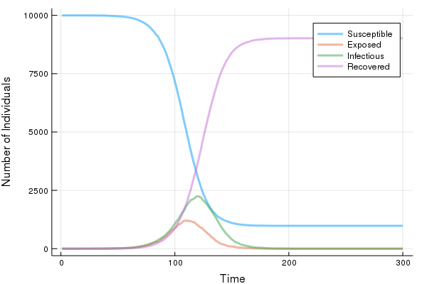
Below is an example simulation where $k^E = 5$, $\gamma^E = 1$, $k^I = 10$, $\gamma^I = 1$, and $\beta_0 = 0.25$ ($R_0 = \beta_0\frac{k^I}{\gamma^I} = 2.5$). The population size is $N = 10,000$. The simmulation starts with 1 exposed case and everyone else belongs to the susceptible class. These settings are the same the the simulation 11 of the original paper.
N.B. Since this is a stochastic model, there is chance for the outbreak not to occur even with a high $R_0$.
sim = seir_simulation( Dict("S" => 9999, "E" => 1, "I" => 0, "R" => 0),
                       Dict("k_E" =>  5, "gamma_E" => 1.0,
                            "k_I" => 10, "gamma_I" => 1.0,
                            "beta" => 0.25),
                       300 )
print(sim[end - 9 : end, :])
10×5 DataFrames.DataFrame
│ Row │ S   │ E │ I │ R    │ time │
├─────┼─────┼───┼───┼──────┼──────┤
│ 1   │ 981 │ 0 │ 0 │ 9019 │ 291  │
│ 2   │ 981 │ 0 │ 0 │ 9019 │ 292  │
│ 3   │ 981 │ 0 │ 0 │ 9019 │ 293  │
│ 4   │ 981 │ 0 │ 0 │ 9019 │ 294  │
│ 5   │ 981 │ 0 │ 0 │ 9019 │ 295  │
│ 6   │ 981 │ 0 │ 0 │ 9019 │ 296  │
│ 7   │ 981 │ 0 │ 0 │ 9019 │ 297  │
│ 8   │ 981 │ 0 │ 0 │ 9019 │ 298  │
│ 9   │ 981 │ 0 │ 0 │ 9019 │ 299  │
│ 10  │ 981 │ 0 │ 0 │ 9019 │ 300  │
Visualisation
gr(fmt = :png)
plot( sim[:, :time],
       [sim[:, :S], sim[:, :E], sim[:, :I], sim[:, :R]],
       label = ["Susceptible", "Exposed", "Infectious", "Recovered"],
       xlabel = "Time", ylabel = "Number of Individuals",
       linealpha = 0.5, linewidth = 3 )
Test Case
srand(12345)
test_sim = seir_simulation( Dict("S" => 9999, "E" => 1, "I" => 0, "R" => 0),
                            Dict("k_E" =>  5, "gamma_E" => 1.0,
                                 "k_I" => 10, "gamma_I" => 1.0,
                                 "beta" => 0.25),
                            100 )
test_result = convert(Array, test_sim[end-2 : end, :])

correct_result = [ 6416  1017  1298  1269   98 ;
                   6210  1045  1379  1366   99 ;
                   6010  1086  1442  1462  100 ]

println("\n-------------------")
if correct_result == test_result
    println("    Test PASSED")
else
    println("    Test FAILED")
end
println("-------------------\n")
-------------------
    Test PASSED
-------------------