An individual-based network model to evaluate interventions for controlling pneumococcal transmission
Author:
- Gerry Tonkin-Hill @gtonkinhill
- Alex Zarebski @aezarebski
Date: 2018-10-01
Summary
Karlsson et al. developed a contact network model to evaluate the efficacy of interventions aiming to control pneumococcal transmission. They used demographic data from Sweden during the mid-2000s to estimate model parameters.
In their model individuals are assigned several features: an age, a household, and potentially a class in school/day care. These features then influence the rate of transmission between individuals in the population. Together this defines a stochastic process of the number of people infected. We carry out a simulation of this process and then generate some visualisations of this.
Model and implementation
Initially we need to set the parameters of the model. These are taken from the paper and estimated using Swedish demographic data.
library(ggplot2)
library(data.table)
#transmission rates
transmission.households <- 0.07
transmission.DCCs <- 0.04
transmission.school.classes <- 0.03
transmission.other.contacts <- 0.04

#age bias
age.bias.1 <- 1
age.bias.1to6 <- 0.33
age.bias.7to65 <- 0.18
age.bias.65 <- 0.3

prop.children.attending.DCCs <- 0.79
average.group.size.DCC <- 16.7
average.class.size.school <- 22
probability.of.other.contacts <- 0.5

pop.size <- 5000
n.initial.carriers <- 125
stop.time <- 156

#sweden population pyramid
sweden.pop.props <- c(2.9,2.9,2.7,2.4,3.4,3.4,3.1,3,3.1,3.5,3.1,2.9,2.7,3.2,2.6,1.9,1.4,1,0.6,0.1,0)
names(sweden.pop.props) <- c(seq(0,100,5)[-1], "100+")

#sweden family size proportions
num.siblings.props <- c(0.19,0.48,0.23,0.10)
names(num.siblings.props) <- c(0,1,2,3)
prop.single.parent <- 0.19
We now give the individuals in the simulation an age as well as assign them to schools, families and day care centres (DCC’s) where appropriate.
pop.ages <- as.numeric(sample(names(sweden.pop.props), pop.size, replace = TRUE, prob = sweden.pop.props))
family.membership <- rep(NA, pop.size)
school.membership <- rep(NA, pop.size)
dcc.membership <- rep(NA, pop.size)
other.close.contact.pair <- rep(NA, pop.size)

#randomly assign an individual a close contact with probability 0.5.
npairs <- rbinom(1, pop.size, 0.5)
pairs <- matrix(sample(pop.size, 2*npairs, replace = TRUE), ncol=2)

#assign families
fam.id <- 1
while(sum(is.na(family.membership[pop.ages<=20]))>0){ #we still have un-assigned children
  n.children <- sample(as.numeric(names(num.siblings.props)), 1, prob=num.siblings.props) + 1
  child.index <- which((pop.ages<=20) & is.na(family.membership))[1:n.children]
  n.parents <- sample(c(1,2), 1, prob = c(prop.single.parent, 1-prop.single.parent))
  parent.index <- which((pop.ages>20) & (pop.ages<=50) & is.na(family.membership))[1:n.parents]
  family.membership[c(child.index, parent.index)] <- fam.id
  fam.id <- fam.id + 1
}

#assign dcc
dcc.id <- 1
n.under.5 <- sum(pop.ages<=5)
indexs.in.dcc <- sample(which(pop.ages<=5), size = floor(prop.children.attending.DCCs*n.under.5))
family.ids <-  unique(family.membership[indexs.in.dcc])
dcc.size <- 0
for(f in family.ids){
  index <- indexs.in.dcc[family.membership[indexs.in.dcc]==f]
  dcc.membership[index] <- dcc.id
  dcc.size <- dcc.size + length(index)
  if(dcc.size>average.group.size.DCC){
    dcc.size <- 0
    dcc.id <- dcc.id + 1
  }
}

#assign schools
#5 to 10
class.id <- 1
indexes.in.school <- which((pop.ages>5) & (pop.ages<=10))
family.ids <-  unique(family.membership[indexes.in.school])
class.size <- 0
for(f in family.ids){
  index <- indexes.in.school[family.membership[indexes.in.school]==f]
  school.membership[index] <- class.id
  class.size <- class.size + length(index)
  if(class.size>average.class.size.school){
    class.size <- 0
    class.id <- class.id + 1
  }
}

#10 to 15yrs
indexes.in.school <- which((pop.ages>10) & (pop.ages<=15))
family.ids <-  unique(family.membership[indexes.in.school])
class.size <- 0
for(f in family.ids){
  index <- indexes.in.school[family.membership[indexes.in.school]==f]
  school.membership[index] <- class.id
  class.size <- class.size + length(index)
  if(class.size>average.class.size.school){
    class.size <- 0
    class.id <- class.id + 1
  }
}
After we’ve assigned individuals to groups we need to set the rate of transmission between people.
transition.matrix <- matrix(1, nrow = pop.size, ncol = pop.size)
#household transmission
for(f in unique(family.membership[!is.na(family.membership)])){
  index <- which(family.membership==f)
  transition.matrix[t(combn(index, 2))] <- transition.matrix[t(combn(index, 2))] * (
    1 - transmission.households)
}

#dcc transmission
for(f in unique(dcc.membership[!is.na(dcc.membership)])){
  index <- which(dcc.membership==f)
  transition.matrix[t(combn(index, 2))] <- transition.matrix[t(combn(index, 2))] * (
    1 - transmission.DCCs)
}

#school transmission
for(f in unique(school.membership[!is.na(school.membership)])){
  index <- which(school.membership==f)
  transition.matrix[t(combn(index, 2))] <- transition.matrix[t(combn(index, 2))] * (
    1 - transmission.school.classes)
}

#other transmission
transition.matrix[pairs] <- transition.matrix[pairs] * (1 - transmission.other.contacts)
transition.matrix[pairs[,c(2,1)]] <- transition.matrix[pairs[,c(2,1)]] * (1 - transmission.other.contacts)

#bias probability vector
bias.probs <- rep(NA, pop.size)
bias.probs[pop.ages<=5] <- 0.33
bias.probs[pop.ages>65] <- 0.3
bias.probs[is.na(bias.probs)] <- 0.18
Now lets simulate! We assume a slightly simpler carriage duration of Poisson with mean 4 weeks.
status.vector <- rep(0, pop.size)
remaining.carriage <- rep(0, pop.size)

#initialise infections
index <- sample(pop.size, n.initial.carriers)
status.vector[index] <- 1
remaining.carriage[index] <- rpois(n = n.initial.carriers, lambda = 4)

pop.ages.factor <- factor(pop.ages)
n.infected.vector <- rep(NA, stop.time)
n.infected.age.matrix <- matrix(NA, nrow = stop.time, ncol = length(unique(pop.ages.factor)))
colnames(n.infected.age.matrix) <- levels(pop.ages.factor)

for(t in 1:stop.time){
  # message(paste("Time:", t))

  prob.infection <- 1-exp(rowSums(log((1-status.vector) * transition.matrix)))
  prob.infection <- prob.infection*bias.probs
  is.infected <- runif(pop.size)<prob.infection

  n.new.infections <- sum((status.vector<=0) & is.infected)
  remaining.carriage[(status.vector<=0) & is.infected] <- rpois(n = n.new.infections, lambda = 4) + 1
  status.vector <- is.infected
  remaining.carriage <- remaining.carriage-1
  remaining.carriage[remaining.carriage<0] <- 0
  status.vector[remaining.carriage<=0] <- 0

  n.infected.vector[[t]] <- sum(status.vector)

  n.infected.age.matrix[t,] <- table(pop.ages.factor[status.vector==1])

}
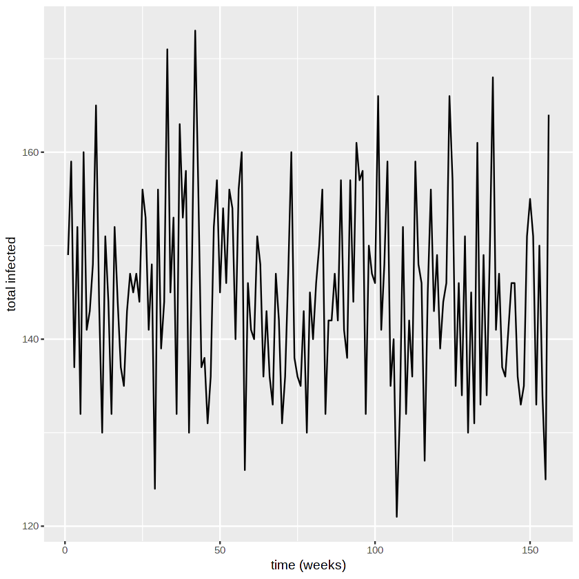
We plot the number of people infected over time.
plot.df <- data.frame(time=1:stop.time, total.infected=n.infected.vector,
                      stringsAsFactors = FALSE)

ggplot(plot.df, aes(x=time, y=total.infected)) +
  geom_line() + xlab("time (weeks)") + ylab("total infected")
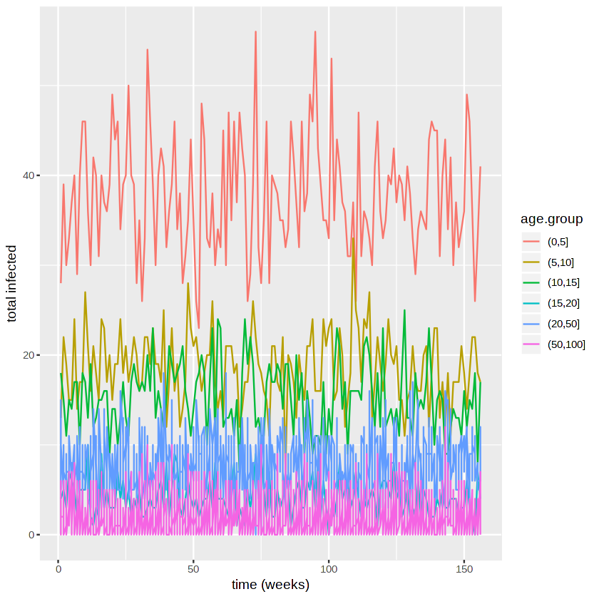
We plot the incidence in different age groups.
plot.df <- melt(n.infected.age.matrix)
colnames(plot.df) <- c("time", "age.group", "number infected")
plot.df$age.group <- cut(plot.df$age.group, breaks = c(0,5,10,15,20,50,100))

ggplot(plot.df, aes(x=time, y=`number infected`, col=age.group)) +
  geom_line() +
  xlab("time (weeks)") + ylab("total infected")
We can compare this to the number in each group.
table(cut(pop.ages, breaks = c(0,5,10,15,20,50,100)))
   (0,5]   (5,10]  (10,15]  (15,20]  (20,50] (50,100]
     339      282      243      214     1970     1952