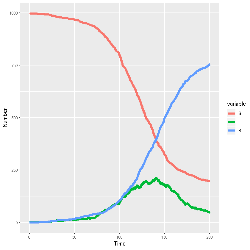
Stochastic SIR model (discrete state, continuous time) in R using GillespieSSA
library(GillespieSSA)
library(reshape2)
a <- c("beta*S*I","gamma*I")
nu <- matrix(c(-1,+1,0,0,-1,+1),nrow=3,ncol=2,byrow=FALSE)
# GillespieSSA
parms <- c(beta=0.1/1000,gamma=0.05)
x0 <- c(S=999,I=1,R=0)
tf <- 200
set.seed(42)
sir_out <- ssa(x0,a,nu,parms,tf=tf,simName="SIR")
while(sir_out$stats$nSteps==1){
    sir_out <- ssa(x0,a,nu,parms,tf=tf,simName="SIR")
}
head(sir_out$data)
| <th scope=col></th><th scope=col>S</th><th scope=col>I</th><th scope=col>R</th> | |||
|---|---|---|---|
| 0.000000 | 999 | 1 | 0 |
| 1.239429 | 998 | 2 | 0 |
| 3.427902 | 997 | 3 | 0 |
| 7.892282 | 997 | 2 | 1 |
| 9.059502 | 996 | 3 | 1 |
| 9.794212 | 995 | 4 | 1 |
sir_out_long <- melt(as.data.frame(sir_out$data),"V1")
Visualisation
library(ggplot2)
ggplot(sir_out_long,aes(x=V1,y=value,colour=variable,group=variable))+
  # Add line
  geom_line(lwd=2)+
  #Add labels
  xlab("Time")+ylab("Number")