Stochastic SIR model with Python
Libraries
import numpy as np
import math
import pandas as pd
import pythran
%%writefile .pythranrc
[compiler]
include_dirs=/usr/include/openblas
Writing .pythranrc
%load_ext pythran.magic
np.random.seed(123)
Plain Python version
def sir(u,parms,t):
    bet,gamm,iota,N,dt=parms
    S,I,R,Y=u
    lambd = bet*(I+iota)/N
    ifrac = 1.0 - math.exp(-lambd*dt)
    rfrac = 1.0 - math.exp(-gamm*dt)
    infection = np.random.binomial(S,ifrac)
    recovery = np.random.binomial(I,rfrac)
    return [S-infection,I+infection-recovery,R+recovery,Y+infection]

def simulate():
    parms = [0.1, 0.05, 0.01, 1000.0, 0.1]
    tf = 200
    tl = 2001
    t = np.linspace(0,tf,tl)
    S = np.zeros(tl)
    I = np.zeros(tl)
    R = np.zeros(tl)
    Y = np.zeros(tl)
    u = [999,1,0,0]
    S[0],I[0],R[0],Y[0] = u
    for j in range(1,tl):
        u = sir(u,parms,t[j])
        S[j],I[j],R[j],Y[j] = u
    return {'t':t,'S':S,'I':I,'R':R,'Y':Y}
%timeit simulate()
8.89 ms ± 85.7 µs per loop (mean ± std. dev. of 7 runs, 100 loops each)
sir_out = pd.DataFrame(simulate())
sir_out
| t | S | I | R | Y | |
|---|---|---|---|---|---|
| 0 | 0.0 | 999.0 | 1.0 | 0.0 | 0.0 |
| 1 | 0.1 | 999.0 | 1.0 | 0.0 | 0.0 |
| 2 | 0.2 | 999.0 | 1.0 | 0.0 | 0.0 |
| 3 | 0.3 | 999.0 | 1.0 | 0.0 | 0.0 |
| 4 | 0.4 | 999.0 | 1.0 | 0.0 | 0.0 |
| 5 | 0.5 | 999.0 | 1.0 | 0.0 | 0.0 |
| 6 | 0.6 | 999.0 | 1.0 | 0.0 | 0.0 |
| 7 | 0.7 | 999.0 | 1.0 | 0.0 | 0.0 |
| 8 | 0.8 | 999.0 | 1.0 | 0.0 | 0.0 |
| 9 | 0.9 | 999.0 | 1.0 | 0.0 | 0.0 |
| 10 | 1.0 | 999.0 | 1.0 | 0.0 | 0.0 |
| 11 | 1.1 | 999.0 | 1.0 | 0.0 | 0.0 |
| 12 | 1.2 | 999.0 | 1.0 | 0.0 | 0.0 |
| 13 | 1.3 | 999.0 | 1.0 | 0.0 | 0.0 |
| 14 | 1.4 | 999.0 | 1.0 | 0.0 | 0.0 |
| 15 | 1.5 | 999.0 | 1.0 | 0.0 | 0.0 |
| 16 | 1.6 | 999.0 | 1.0 | 0.0 | 0.0 |
| 17 | 1.7 | 999.0 | 1.0 | 0.0 | 0.0 |
| 18 | 1.8 | 999.0 | 1.0 | 0.0 | 0.0 |
| 19 | 1.9 | 999.0 | 1.0 | 0.0 | 0.0 |
| 20 | 2.0 | 999.0 | 1.0 | 0.0 | 0.0 |
| 21 | 2.1 | 999.0 | 1.0 | 0.0 | 0.0 |
| 22 | 2.2 | 999.0 | 1.0 | 0.0 | 0.0 |
| 23 | 2.3 | 999.0 | 1.0 | 0.0 | 0.0 |
| 24 | 2.4 | 999.0 | 1.0 | 0.0 | 0.0 |
| 25 | 2.5 | 999.0 | 1.0 | 0.0 | 0.0 |
| 26 | 2.6 | 999.0 | 1.0 | 0.0 | 0.0 |
| 27 | 2.7 | 999.0 | 1.0 | 0.0 | 0.0 |
| 28 | 2.8 | 999.0 | 1.0 | 0.0 | 0.0 |
| 29 | 2.9 | 999.0 | 1.0 | 0.0 | 0.0 |
| ... | ... | ... | ... | ... | ... |
| 1971 | 197.1 | 285.0 | 62.0 | 653.0 | 714.0 |
| 1972 | 197.2 | 285.0 | 62.0 | 653.0 | 714.0 |
| 1973 | 197.3 | 285.0 | 62.0 | 653.0 | 714.0 |
| 1974 | 197.4 | 285.0 | 61.0 | 654.0 | 714.0 |
| 1975 | 197.5 | 285.0 | 60.0 | 655.0 | 714.0 |
| 1976 | 197.6 | 285.0 | 60.0 | 655.0 | 714.0 |
| 1977 | 197.7 | 285.0 | 59.0 | 656.0 | 714.0 |
| 1978 | 197.8 | 285.0 | 58.0 | 657.0 | 714.0 |
| 1979 | 197.9 | 285.0 | 57.0 | 658.0 | 714.0 |
| 1980 | 198.0 | 285.0 | 57.0 | 658.0 | 714.0 |
| 1981 | 198.1 | 285.0 | 57.0 | 658.0 | 714.0 |
| 1982 | 198.2 | 285.0 | 57.0 | 658.0 | 714.0 |
| 1983 | 198.3 | 285.0 | 57.0 | 658.0 | 714.0 |
| 1984 | 198.4 | 285.0 | 57.0 | 658.0 | 714.0 |
| 1985 | 198.5 | 285.0 | 56.0 | 659.0 | 714.0 |
| 1986 | 198.6 | 285.0 | 56.0 | 659.0 | 714.0 |
| 1987 | 198.7 | 285.0 | 55.0 | 660.0 | 714.0 |
| 1988 | 198.8 | 284.0 | 56.0 | 660.0 | 715.0 |
| 1989 | 198.9 | 284.0 | 56.0 | 660.0 | 715.0 |
| 1990 | 199.0 | 282.0 | 58.0 | 660.0 | 717.0 |
| 1991 | 199.1 | 282.0 | 58.0 | 660.0 | 717.0 |
| 1992 | 199.2 | 282.0 | 57.0 | 661.0 | 717.0 |
| 1993 | 199.3 | 282.0 | 57.0 | 661.0 | 717.0 |
| 1994 | 199.4 | 282.0 | 57.0 | 661.0 | 717.0 |
| 1995 | 199.5 | 282.0 | 57.0 | 661.0 | 717.0 |
| 1996 | 199.6 | 282.0 | 56.0 | 662.0 | 717.0 |
| 1997 | 199.7 | 282.0 | 55.0 | 663.0 | 717.0 |
| 1998 | 199.8 | 281.0 | 56.0 | 663.0 | 718.0 |
| 1999 | 199.9 | 281.0 | 55.0 | 664.0 | 718.0 |
| 2000 | 200.0 | 281.0 | 54.0 | 665.0 | 718.0 |
2001 rows × 5 columns
Pythran compiled version
As the above code only uses simple Python and Numpy times, it is straightforward to obtain compiled versions of the code using Pythran.
%%pythran -DUSE_XSIMD -march=native -O3

import numpy as np
import math

#pythran export sirp(float64 list, float64 list, float64)
def sirp(u,parms,t):
    bet,gamm,iota,N,dt=parms
    S,I,R,Y=u
    lambd = bet*(I+iota)/N
    ifrac = 1.0 - math.exp(-lambd*dt)
    rfrac = 1.0 - math.exp(-gamm*dt)
    infection = np.random.binomial(S,ifrac)
    recovery = np.random.binomial(I,rfrac)
    return [S-infection,I+infection-recovery,R+recovery,Y+infection]

#pythran export simulatep()
def simulatep():
    parms = [0.1, 0.05, 0.01, 1000.0, 0.1]
    tf = 200
    tl = 2001
    t = np.linspace(0,tf,tl)
    S = np.zeros(tl)
    I = np.zeros(tl)
    R = np.zeros(tl)
    Y = np.zeros(tl)
    u = [999,1,0,0]
    S[0],I[0],R[0],Y[0] = u
    for j in range(1,tl):
        u = sirp(u,parms,t[j])
        S[j],I[j],R[j],Y[j] = u
    return {'t':t,'S':S,'I':I,'R':R,'Y':Y}
%timeit simulatep()
434 µs ± 18.3 µs per loop (mean ± std. dev. of 7 runs, 1000 loops each)
This is around two orders of magnitude faster than the vanilla Python code.
sir_outp = pd.DataFrame(simulatep())
sir_outp
| Y | R | I | S | t | |
|---|---|---|---|---|---|
| 0 | 0.0 | 0.0 | 1.0 | 999.0 | 0.0 |
| 1 | 0.0 | 0.0 | 1.0 | 999.0 | 0.1 |
| 2 | 0.0 | 0.0 | 1.0 | 999.0 | 0.2 |
| 3 | 0.0 | 0.0 | 1.0 | 999.0 | 0.3 |
| 4 | 0.0 | 0.0 | 1.0 | 999.0 | 0.4 |
| 5 | 0.0 | 0.0 | 1.0 | 999.0 | 0.5 |
| 6 | 0.0 | 0.0 | 1.0 | 999.0 | 0.6 |
| 7 | 0.0 | 0.0 | 1.0 | 999.0 | 0.7 |
| 8 | 0.0 | 0.0 | 1.0 | 999.0 | 0.8 |
| 9 | 0.0 | 0.0 | 1.0 | 999.0 | 0.9 |
| 10 | 0.0 | 0.0 | 1.0 | 999.0 | 1.0 |
| 11 | 0.0 | 0.0 | 1.0 | 999.0 | 1.1 |
| 12 | 0.0 | 0.0 | 1.0 | 999.0 | 1.2 |
| 13 | 0.0 | 0.0 | 1.0 | 999.0 | 1.3 |
| 14 | 0.0 | 0.0 | 1.0 | 999.0 | 1.4 |
| 15 | 0.0 | 0.0 | 1.0 | 999.0 | 1.5 |
| 16 | 0.0 | 0.0 | 1.0 | 999.0 | 1.6 |
| 17 | 0.0 | 1.0 | 0.0 | 999.0 | 1.7 |
| 18 | 0.0 | 1.0 | 0.0 | 999.0 | 1.8 |
| 19 | 0.0 | 1.0 | 0.0 | 999.0 | 1.9 |
| 20 | 0.0 | 1.0 | 0.0 | 999.0 | 2.0 |
| 21 | 0.0 | 1.0 | 0.0 | 999.0 | 2.1 |
| 22 | 0.0 | 1.0 | 0.0 | 999.0 | 2.2 |
| 23 | 0.0 | 1.0 | 0.0 | 999.0 | 2.3 |
| 24 | 0.0 | 1.0 | 0.0 | 999.0 | 2.4 |
| 25 | 0.0 | 1.0 | 0.0 | 999.0 | 2.5 |
| 26 | 0.0 | 1.0 | 0.0 | 999.0 | 2.6 |
| 27 | 0.0 | 1.0 | 0.0 | 999.0 | 2.7 |
| 28 | 0.0 | 1.0 | 0.0 | 999.0 | 2.8 |
| 29 | 0.0 | 1.0 | 0.0 | 999.0 | 2.9 |
| ... | ... | ... | ... | ... | ... |
| 1971 | 0.0 | 1.0 | 0.0 | 999.0 | 197.1 |
| 1972 | 0.0 | 1.0 | 0.0 | 999.0 | 197.2 |
| 1973 | 0.0 | 1.0 | 0.0 | 999.0 | 197.3 |
| 1974 | 0.0 | 1.0 | 0.0 | 999.0 | 197.4 |
| 1975 | 0.0 | 1.0 | 0.0 | 999.0 | 197.5 |
| 1976 | 0.0 | 1.0 | 0.0 | 999.0 | 197.6 |
| 1977 | 0.0 | 1.0 | 0.0 | 999.0 | 197.7 |
| 1978 | 0.0 | 1.0 | 0.0 | 999.0 | 197.8 |
| 1979 | 0.0 | 1.0 | 0.0 | 999.0 | 197.9 |
| 1980 | 0.0 | 1.0 | 0.0 | 999.0 | 198.0 |
| 1981 | 0.0 | 1.0 | 0.0 | 999.0 | 198.1 |
| 1982 | 0.0 | 1.0 | 0.0 | 999.0 | 198.2 |
| 1983 | 0.0 | 1.0 | 0.0 | 999.0 | 198.3 |
| 1984 | 0.0 | 1.0 | 0.0 | 999.0 | 198.4 |
| 1985 | 0.0 | 1.0 | 0.0 | 999.0 | 198.5 |
| 1986 | 0.0 | 1.0 | 0.0 | 999.0 | 198.6 |
| 1987 | 0.0 | 1.0 | 0.0 | 999.0 | 198.7 |
| 1988 | 0.0 | 1.0 | 0.0 | 999.0 | 198.8 |
| 1989 | 0.0 | 1.0 | 0.0 | 999.0 | 198.9 |
| 1990 | 0.0 | 1.0 | 0.0 | 999.0 | 199.0 |
| 1991 | 0.0 | 1.0 | 0.0 | 999.0 | 199.1 |
| 1992 | 0.0 | 1.0 | 0.0 | 999.0 | 199.2 |
| 1993 | 0.0 | 1.0 | 0.0 | 999.0 | 199.3 |
| 1994 | 0.0 | 1.0 | 0.0 | 999.0 | 199.4 |
| 1995 | 0.0 | 1.0 | 0.0 | 999.0 | 199.5 |
| 1996 | 0.0 | 1.0 | 0.0 | 999.0 | 199.6 |
| 1997 | 0.0 | 1.0 | 0.0 | 999.0 | 199.7 |
| 1998 | 0.0 | 1.0 | 0.0 | 999.0 | 199.8 |
| 1999 | 0.0 | 1.0 | 0.0 | 999.0 | 199.9 |
| 2000 | 0.0 | 1.0 | 0.0 | 999.0 | 200.0 |
2001 rows × 5 columns
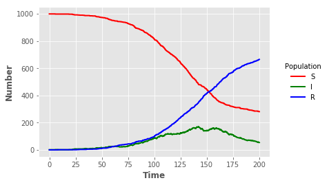
Visualisation
import matplotlib.pyplot as plt
plt.style.use("ggplot")
sline = plt.plot("t","S","",data=sir_out,color="red",linewidth=2)
iline = plt.plot("t","I","",data=sir_out,color="green",linewidth=2)
rline = plt.plot("t","R","",data=sir_out,color="blue",linewidth=2)
plt.xlabel("Time",fontweight="bold")
plt.ylabel("Number",fontweight="bold")
legend = plt.legend(title="Population",loc=5,bbox_to_anchor=(1.25,0.5))
frame = legend.get_frame()
frame.set_facecolor("white")
frame.set_linewidth(0)